Introduction
Detections of image and processing artifacts in image differencing present a significant challenge to LSST’s recovery of faint moving objects. The task of the moving objects pipeline is to take all detections of new or changed sources in a set of images and identify which of these detections can be linked together as repeat observations of a single moving object. While linking observations of one object may be simple, the difficulty comes from rejecting every other combination of detections. These detections may come from other moving objects, or from astrophysical transients outside the Solar System, or from imaging and data processing artifacts. All of these sources of candidate detections contribute a background which the moving objects pipeline must search through in order to correctly link object tracks.
All asteroid surveys must rely on both their observing cadence and their data processing to enable detection of moving objects. For LSST, in the baseline cadence the scheduler attempts to visit fields twice within 90 minutes. These visits within one night produce a set of “tracklets” between every combination of detections that have separations corresponding to reasonable Solar System object velocities. This linkage is relatively simple, but tracklets must then be linked into multi-night tracks. This is the most computationally-intensive step in the process, since numerous combinations of tracklets must checked to see if their motion is consistent with an orbit (quadratic motion with reasonable acceleration; also see LDM-156).
Previous searches for asteroids have found that the vast majority of candidate detections are caused by imaging or processing artifacts, which leads to an excess of tracklets and an excessive computational cost for distinguishing real tracks. In the case of Pan-STARRS, the false positive rate of \(8,000\) per square degree necessitated additional observations of each field in a single night, so that true objects would have tracklets with three or more detections (Denneau et al. 2013). The Dark Energy Survey, while mainly searching for transients rather than moving solar system objects, employed machine learning algorithms to exclude detections that were unlikely to be physical (Kessler et al. 2015, Goldstein et al. 2015).
The goal of this study is to quantify the expected rate of false positive detections in LSST, using the LSST image differencing pipeline run on observations taken with Decam. Producing clean difference images is a substantial software challenge. As described in LSST reports (Becker et al. Winter 2013 report) and published works (Alard & Lupton 1991), the convolution process required to match the point spread functions of the two images (PSFs) introduces correlated noise which complicates detection. Improved algorithms for image subtraction are still an active area of research (Zackay et al. 2015). Our objective is to characterize the performance of the current pipeline with the understanding that it will be improved in the time leading up to the start of operations.
Data and Pipeline Processing
The observations used in this work were part of a near Earth object (NEO) search program conducted in 2013 (Program 2013A-724, PI: L. Allen). The data are publicly available in the NOAO archive, and a table of the individual exposures used can be found in Appendix A. These exposures are a small subset of the full observing program. The full set of exposures was divided into five bands in absolute Galactic latitude, a single field in each range was randomly chosen and all observations of that field were downloaded. The input to the LSST pipeline were “InstCal” files for which instrumental signature removal (ISR) had been applied by the NOAO Community Pipeline. This stage of processing is very instrument-specific and the LSST pipeline had only a limited ability to apply ISR to Decam images at the time.
The LSST pipeline was used to background subtract the images, compute the PSF,
and perform photometry (all conducted by processCcdDecam.py). Astrometric
calibration was provided by the Community Pipeline values; we did not re-fit
the astrometry [1]. In each field one image was selected to serve as the
“template” against which all other observations in that field would be
differenced. This was done by imageDifference.py, which computed the
matching kernel, convolved and warped the template to match the non-template
exposure and performed the subtraction. Existing default settings were used
throughout. Source detection was performed at the \(5.0\sigma\) level.
Dipole fitting and PSF photometry was performed on all detections.
A set of postage stamps showing Dia source detections are shown in Figure 1. The appearance of these is quite varied. Some are clearly the result of poorly subtracted stars, and show both positive and negative artifacts. The dipole fitting code in the LSST pipeline attempts to fit both negative and positive components to a detection, and then flags sources as dipoles if the the absolute value of the flux in both components is similar (neither component holds more than 65% of the total flux). Detections where this flag is set have been marked “Dipole” on the left side of the postage stamps, and one can see that this successfully identifies many of the bright stars with failed subtractions.
Many of the other detections show no apparent source at all in the original images, and the presence of a flux overdensity or underdensity is barely perceptible by eye. Some of these detections could simply be noise excursions that happen to exceed the \(5.0\sigma\) detection threshold. However they could also be real detections of particularly faint objects, and thus it is critical to understand the origin of these detections.
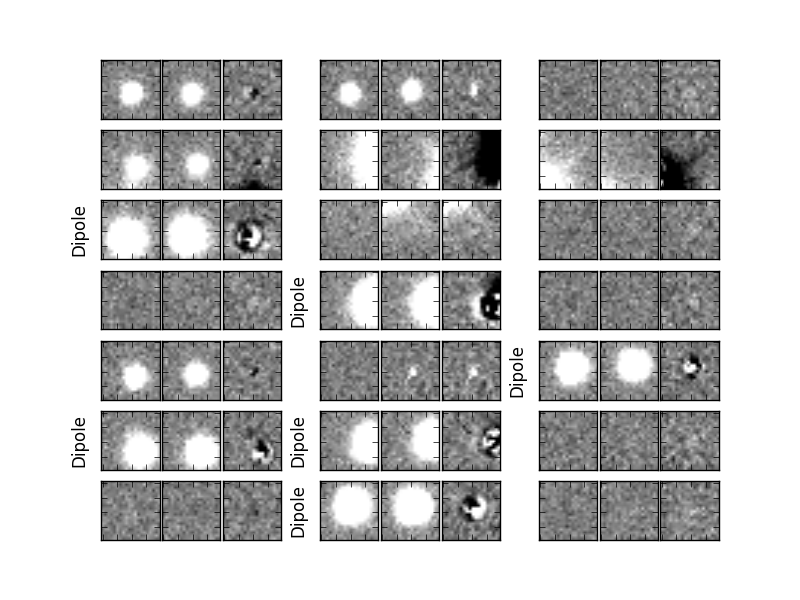
Figure 1 Example postage stamps of Dia sources in visit 197367. For each triplet of images, the left image is the template, the center image is the science exposure, and the right image is the difference. Many of these result from poor subtractions of bright stars, but many are in areas that appear empty.
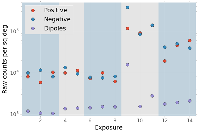
Figure 2 Raw density of DIA sources per square degree, without any filtering, for all exposures in this work. The exposures are arbitrarily numbered and cover several different nights. Each shaded region corresponds to a different target field.
| [1] | We tested the processing both with and without the astrometric distortion terms provided by the Community Pipeline and did not see a significant difference in the numbers of Dia source detections. |
Direct Image Noise Analysis
One check on the pipeline noise estimates can be made by taking two overlapping exposures, crossmatching the detected sources in each, and comparing the difference in the fluxes measured each time with the reported uncertainties on those fluxes. This test is independent of any of image differencing. The reported uncertainties are derived from each exposure’s variance plane, which is also used for computing the uncertainties on the difference images.
Figure 3 shows this analysis performed for a pair of well-behaved fields at high latitude. The scatter in the measured fluxes is about 15% wider than the pipeline uncertainties report. While this is enough to account for ~300 detections per square degree, that still falls fall short of the actual detection numbers we see in the high latitude images.
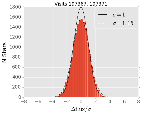
Figure 3 Difference in measured flux between exposures 197367 and 197371, normalized by the reported uncertainty on each measurement. If the reported uncertainties are correct, this should form a unit Gaussian, however it is better fit by a Gaussian that is 15% wider.
The same analysis for one of the visits with extremely high DIA source counts, visit 197662, is shown in Figure 4. In this image the variance plane underestimates the scatter in the photometry by approximately 60%. This will certainly lead to an order of magnitude excess of detections, and we do not investigate these fields further.
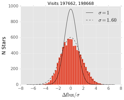
Figure 4 Difference in measured flux between the low latitude exposures 197662 and 198668, normalized by the reported uncertainty on each measurement. In this comparison the reported uncertainties are significantly smaller than the observed scatter in the fluxes, differing by about 60%.
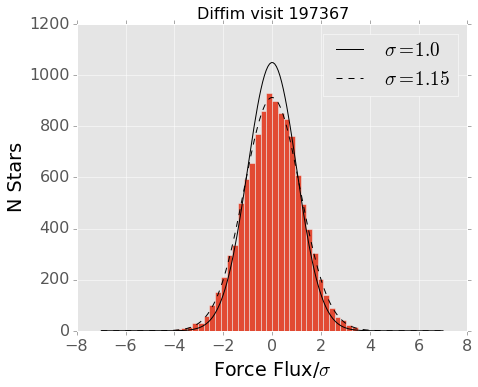
Figure 5 Force photometry on random locations in the difference image. This measures the noise on the same size scale as the PSF. The reported uncertainties are about 15% smaller than the observed scatter. This is consistent with propagating the variance plane provided by the Community Pipeline.
Noise in Difference Images
Even after rescaling the variance planes on the input images, the number of detections per square degree are several orders of magnitude greater than expected from Gaussian noise. For an image with a Gaussian PSF of width \(\sigma_g\) in pixels (note this is the Gaussian \(\sigma\), not the full width at half max), the density of detections above a threshold \(\nu\) is
where the total number per image is
This expectation is described in Kaiser (2004) and Becker et al. (2013). For the Decam images with seeing of \(\sigma_g = 1.8\) pixels and 2k by 4k pixel sensor, we expect 1.5 noise detections per sensor at \(5\sigma\) or 33 detections per square degree (twice that if counting both positive and negative detections). The raw rate we measure is 100 times this. This suggests that either some substantial quantity of artifacts (in the original images or introduced by the LSST software) are present, or that the pipeline’s estimate of the threshold for detection is incorrect.
We believe that latter effect is the dominant contributor of false detections. If the pipeline underestimates the variance in the difference images, then what we call “\(5\sigma\)” will not correspond to our actual intended detection threshold. This true for the direct images as well, but for the difference images the problem of tracking the variance becomes much more difficult due to the convolution steps (Price & Magnier 2004, Becker et al. 2013).
A particularly useful tool for isolating the effects of the differencing pipeline from effects in the original direct images is to perform force photometry (fitting a PSF source amplitude at a fixed position) in the direct images at the location of all DIA sources. A diagram showing the results from this for a single field is shown in Figure 6.
Because we are differencing two single exposures rather than an exposure against a coadd, a source appearing in the science exposure will need to have a signal to noise ratio of \(5\sqrt{2}\) to be detected as a \(5 \sigma\) source in the difference image. The force photometry diagrams thus show this threshold as the two diagonal lines, for positive and negative sources.
Though this should be the threshold for detection, the presence of numerous sources just inside the \(5 \sqrt{2}\sigma\) lines indicates that the pipeline is being overly permissive in detection. The uncertainty on the difference image measurement cannot be less than the uncertainties on the two input images, but the convolution used for matching the PSFs makes it difficult to keep track of this uncertainty. When the pipeline convolves the template image, the variance plane is reduced since the process is essentially Gaussian smoothing. While this does track the diminished per-pixel variance, it does not account for the correlations introduced between adjacent pixels. These untracked correlations will then boost the significance of detections when the difference image is convolved with the detection kernel, resulting in an excess of false positives.
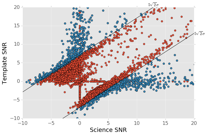
Figure 6 PSF photometry in the template and science exposures, forced on the positions of DIA source detections. The parallel diagonal lines denote \(\rm{science} - \rm{template} > 5\sqrt{2}\sigma\) and \(\rm{science} - \rm{template} < -5 \sqrt{2}\sigma\), which are the intended criteria for detection. The fact that numerous detections appear just inside these lines is a result of the mis-estimation of the variance in the difference image (some incidental failures are also present in this region).
Figure 7 also illustrates this error estimation problem. The panel on the left shows a histogram of the the signal to noise ratio from force photometry on the two input images. This uncertainty estimate involves no image differencing code and should be accurate. The panel on the right shows the pipeline’s reported signal to noise ratio as measured on the difference image, where the difference image variance plane is used to estimate the uncertainty. It is clear that the pipeline reports that its detections are substantially more significant than our direct image estimates. This is entirely due to differences in the reported uncertainties. The ratio of the difference image uncertainty to the sum of the direct image uncertainties is between 0.8 and 0.85 for nearly all sources in this image.
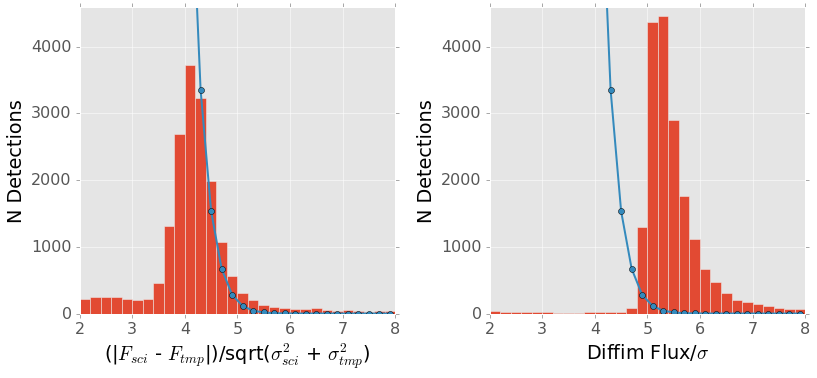
Figure 7 Comparison of force photometry SNR versus the SNR of measurements on the difference image for all sources in one exposure (visit 197367). The blue line shows the expected counts from random noise. When the noise is properly accounted for by force photometry (left), the vast majority of detections are consistent with what we would expect from noise.
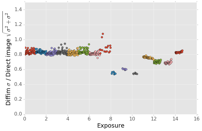
Figure 8 Mean of the ratio of reported uncertainty to expected uncertainty for each CCDs over all visits. While values around 0.8 are generally common, there is some variation from field to field. This is presumably related to the observing conditions in some fashion, but we have not explored the source of this variation.
The problem of correlated noise has been studied before and algorithmic strategies have been proposed for mitigating the issue (Price & Magnier 2010, Becker et al. 2013). These methods require some level of modification to or analysis of the images in the differencing process. We propose that there is a simpler solution that will work equivalently well: the same force photometry measurements that we have used to diagnose this problem may also be used to filter “real” \(5\sigma\) detections from excess of noise detections. This requires little change to the pipeline and can be easily incorporated into the standard processing. The reported measurement would then be the difference of the two PSF fluxes from the direct images, rather than from the difference image. This is a completely equivalent measurement.
| Source Type | Visit 197367 counts per sq. deg | All visits, counts per sq. deg |
|---|---|---|
| Raw Positive Sources | 3,572 | 19,475 |
| Raw Negative Sources | 4,763 | 23,018 |
| Dipoles (not included below) | 1,124 | 1,609 |
| Positive after \(5\sigma\) cut | 480 | 1,022 |
| Negative after \(5\sigma\) cut | 555 | 600 |
| Positive sources excluding “variables” | 237 | 344 |
The results of this process are quantified for a single field in Table 1. The number of detections is reduced by a factor of \(\sim 10\), simply by eliminating all detections that could not possibly be \(5\sigma\). We also compute the density of detections after excluding “variables”, which we use as a broadly-encompassing term for sources that appear at \(>15\sigma\) in both template and science images (this cut-off is arbitrary, but using a limit of of \(>10\sigma\) for example makes very little difference). These are unlikely to be asteroids, although this could potentially be excluding asteroids which appear on top of other sources.
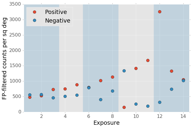
Figure 9 Result of forced photometry \(5\sigma\) cut. The exposure numbering and shading is the same as Figure 2. While some fields apparently developed a bias between negative and positive counts, this is potentially a result of the template selection process.
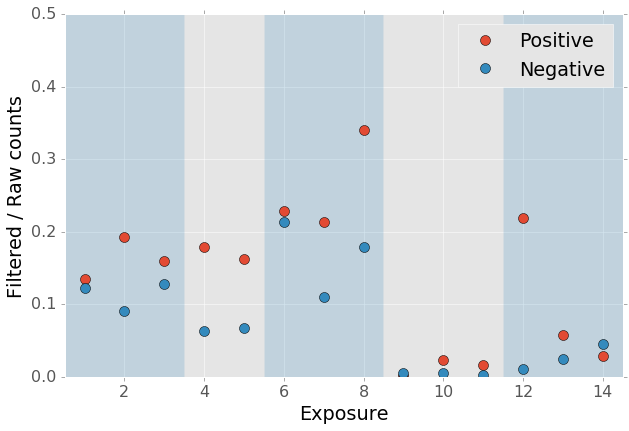
Figure 10 Ratio of the \(5\sigma\) counts to the raw detection counts.
Detections near Bright Stars
In addition to the overall rate of false positives across the each pointing, the spatial distribution of detections present additional challenges to successfully recovering moving objects. Strong correlations between DIA sources can create numerous tracklets of the right length to mimic moving sources. Such correlations are often found around bright stars, where diffraction spikes, increased photon noise from the wings of the star, or minor image misalignments can all result in an excess of DIA sources.
Many of these effects are caused by the telescope optics, and thus our precursor datasets are less likely to precisely capture all of the structure that will be present around bright stars in LSST. However, we can test the LSST software’s ability to mitigate such artifacts, by effective masking, tracking of the per-pixel noise, or other methods.
To compute the distribution of excess detections around bright stars, we cross-matched the UCAC4 catalog of bright stars against the detections in all fields. Figure 11 shows the cumulative count of excess DIA sources as a function of distance from a bright star, with several different magnitude bins for the central star. These curves have had the cumulative counts just from randomly distributed DIA sources subtracted off (on average 2 stars inside a 60 arcsecond radius), leaving only the detections that result from the bright star.
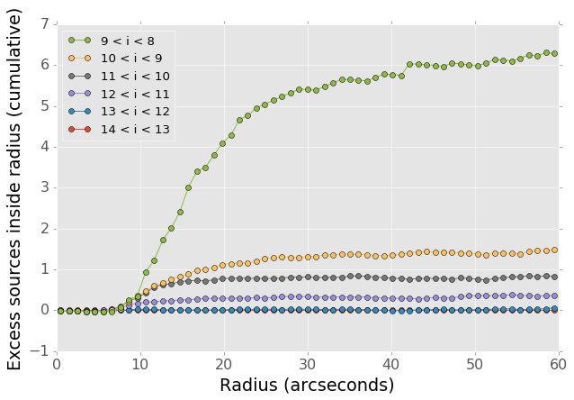
Figure 11 Cumulative distribution of excess detections near bright stars.
Overall the numbers of excess detections are not large; even a 8th magnitude star produces only 8 extra DIA sources, and this number falls off rapidly for fainter stars. These detections all occur outside of 8 arcseconds, since this is the size of the “footprint” that the LSST pipeline assigns to these bright objects. The vast majority of excess detections occur in an annulus between this \(8''\) limit and \(20''\). An example difference image with a bright star is shown in Figure 12. Excess detections are found outside the detection footprint of the bright star, causing the inner hole in Figure 11, but generally inside of \(30''\) from the star.
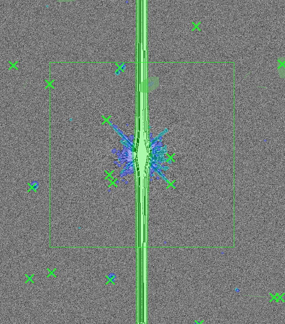
Figure 12 Example difference image around a 7th magnitude star. DIA source detections are marked with green x’s. Green shaded regions are saturated and masked, while blue and cyan shading denotes the extent of a detected “footprint”. The green box is 2 arcminutes on a side. A very bright CCD bleed passes vertically through the star, but is effectively masked.
Figure 13 shows the distribution of SNRs for these excess detections around bright stars as compared to the “normal” detections found across the field. The two curves have been normalized to have the same total number of counts. Both behave very similarly—the bright star sources are not preferentially brighter than those in the field as might be expected if we were detecting diffraction spikes or other bright optical artifacts.
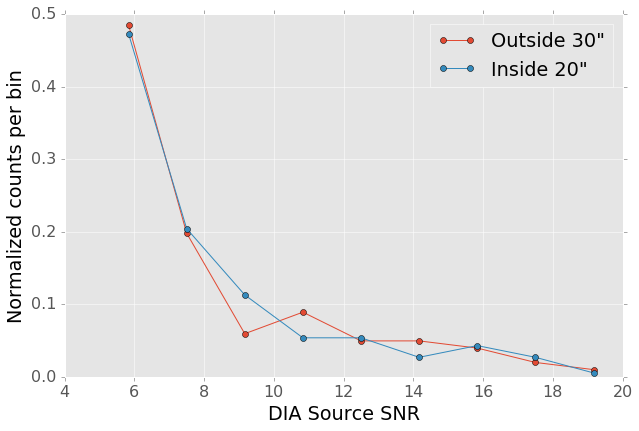
Figure 13 Signal to noise ratio distribution for DIA sources within \(20''\) vs outside of \(30''\) from a bright star (brighter than \(i=11\)). The distributions are normalized to have the same total counts. There is no significant difference in the SNR distribution between the sources around bright stars and the sources that randomly cover the field.
Model of Excess Detections
A simple model for these excess detections is shown in Figure 14. In this we assume a power law for the total number of detections per bright star, as a function of bright star magnitude. An approximate fit for this power law is shown in Figure 15, and the number of counts \(C\) can be written as
where M is the i-band magnitude of the bright star. These detections are then spread uniformly in an annulus around the bright source of size
This puts the outer edge of the detections at \(22''\) for the 9th magnitude case and gradually shrinks the annulus for fainter sources.
While this is certainly not a fit that is accurate to 10%, it is generally within \(\pm 1\) detection. The assumption of a constant density annulus of detections is also imprecise but simple to implement. A density gradient could be added if necessary, but for the purposes of testing the performance of moving object detection we believe this to be sufficient.
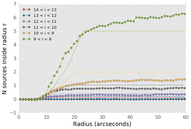
Figure 14 Basic model for the cumulative distribution of counts around bright stars. The model is clearly not precise, but the raw number of counts per stars is so low that we are generally within \(\pm 1\) detection per bright star.
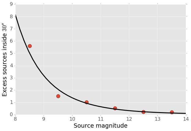
Figure 15 Simple power law model for the number of excess detections inside 30 arcseconds from a bright star.
Uncorrected Artifacts
Visual inspection of exposures have also lead to the discovery of correlated sets of detections, most notably in the crosstalk image of a bright star bleed trail shown in Figure 16. In this case the bright star on the left creates a vertical line of saturated pixels, and when the image is read out, the amplifier reading the right side of the image (without the bleed) is affected by the strong signal on the left side amplifier. While we show this for completeness, in this example dataset the crosstalk corrections that should remove this effect was performed by the Decam Community Pipeline, rather than the LSST software stack. A future extension of this work will be to enable the LSST pipeline’s crosstalk corrections on Decam images and ensure that this effect is properly mitigated.
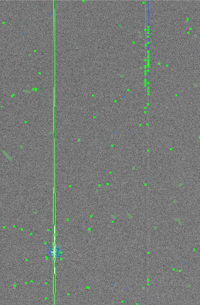
Figure 16 Example detection on the crosstalk image (right side) of a CCD charge bleed (left side vertical line).
Conclusions
The primary result from this work is that the LSST pipeline is capable of producing a clean sample of difference image detections, at roughly the 200-400 per square degree level, as long as the image variance is carefully tracked. In the case of the test data we tried, this required adjusting the variance measures supplied by an external pipeline to match the observed scatter in pixel variance. Similar checks will be necessary when using variance estimates generated by the LSST pipeline, but overall this is relatively simple.
The more complicated challenge is tracking the image variance after convolution, since that process transforms the noise which is purely per-pixel (each pixel is independent) in the input images into a mixture of per-pixel noise and correlated noise between pixels. This correlated noise is not currently tracked by the LSST software, and so the detection process defines a threshold relative to the per-pixel noise level. In our testing this threshold is too low by 20-30%, resulting large numbers of detections with signal to noise ratios between \(4\sigma\) and \(5\sigma\) being reported as \(>5\sigma\) detections.
We present a fix to this mis-estimate by computing the expected uncertainty on DIA sources from force photometry on the input direct images. This uses the convolved difference image for detection, but avoids any dependence on the variance reported from convolved images.
An alternative method is to estimate the effective variance (including both per pixel and PSF-scale covariance) in difference images from force photometry on blank patches of sky. We believe that this is an equivalently effective method and will also be useful for quality assurance. Our choice of implementing force photometry on detections should be understood as an expedient proof of concept rather than a final design decision.
Further work
There are a number of ways in which this effort could be extended. Some of these are:
- Testing on deeper exposures. The data currently used are 60 second exposures on a 4 meter telescope. Scaling by the collecting area, this is about 65% of the depth of an LSST visit. While we expect that many CCD artifacts should not be strongly dependent on the exposure depth, the number of astrophysical sources in the images will be increased and consequently so will the possibility of mis-subtracted sources appearing in the difference images.
- Differencing against coadded templates. The tests in this work were done on differences between single exposures. The baseline procedure for LSST will be to build template images by coadding the exposures taken over some recent time period. This reduces the noise and permits deeper detection of transient sources. However, coadded templates may also retain the sum total of all uncorrected artifacts from their constituent exposures, if these features are not properly masked or otherwise accounted for.
- Instrument rotation. Since the CTIO 4-meter telescope has a equatorial mount, the detectors are always oriented in the same direction on the sky between visits. Features like diffraction spikes and CCD charge bleeds thus overlap each other in subsequent visits. In an alt-az mounted telescope like LSST, images from visits at different hour angles will be rotated relative to each other, and this may create a more complicate structure of image artifacts. Testing the LSST pipeline’s behavior in this situation requires data from an alt-az telescope. Subaru is perhaps the best candidate for this, given its high level of support in the LSST pipeline.
- Dependence on source density, Galactic latitude, sky background, or other observing parameters. Our results for this sample of images show considerable variation in their properties, and we have not attempted to model the behavior of individual exposures. Extending the set of sample images to test the image differencing pipeline in a wide variety of conditions will provide valuable information for both modeling the false positive behavior and for improving the pipeline in general.
Appendix A: Data used in this work
The data used were taken as part of a a NEO search on the CTIO 4-meter, Program 2013A-724, PI: L. Allen. All exposures were 60 seconds.
| Visit | Template | Time Observed | CCDs | Galactic Lat | Galactic Lon |
|---|---|---|---|---|---|
| 197371 | 2013-04-16 00:18:45 | ||||
| 197367 | 197371 | 2013-04-16 00:12:53 | 59 | 56.3311 | 297.6941 |
| 197375 | 197371 | 2013-04-16 00:24:42 | 59 | 56.3355 | 298.0934 |
| 197379 | 197371 | 2013-04-16 00:30:35 | 59 | 56.3461 | 297.6202 |
| 197384 | 2013-04-16 00:40:02 | ||||
| 197388 | 197384 | 2013-04-16 00:45:58 | 59 | 46.0518 | 308.6413 |
| 197392 | 197384 | 2013-04-16 00:51:58 | 59 | 46.0973 | 308.8498 |
| 197408 | 2013-04-16 01:15:18 | ||||
| 197400 | 197408 | 2013-04-16 01:03:24 | 59 | 43.9119 | 312.3330 |
| 197404 | 197408 | 2013-04-16 01:09:21 | 59 | 43.9128 | 312.3235 |
| 197412 | 197408 | 2013-04-16 01:21:18 | 54 | 43.8827 | 312.2617 |
| 197790 | 2013-04-16 23:15:06 | ||||
| 197802 | 197790 | 2013-04-16 23:32:55 | 7 | -22.8796 | 211.1369 |
| 198380 | 197790 | 2013-04-17 23:23:11 | 7 | -22.9299 | 211.1618 |
| 198384 | 197790 | 2013-04-17 23:29:07 | 7 | -22.8802 | 211.1440 |
| 197662 | 2013-04-16 10:03:03 | ||||
| 198668 | 197662 | 2013-04-18 08:37:43 | 47 | -34.6799 | 39.8085 |
| 199009 | 197662 | 2013-04-19 09:32:02 | 37 | -34.5272 | 39.9427 |
| 199021 | 197662 | 2013-04-19 09:50:28 | 37 | -34.5853 | 40.0062 |
| 199033 | 197662 | 2013-04-19 10:08:32 | 23 | -34.7855 | 40.1130 |